My Learnings in ML

Lets talk about one of the difficult areas in ML - Deep Reinforcement Learning. Two of the most popularly used approaches in the space policy gradients and deep Q-networks . An agent interacts with the user within an environment and receives rewards . Policy search is finding a good set of parameters in the policy space . One way to explore the policy space is via policy gradient approach which evaluates the gradients of the rewards w.r.t the parameters and then moves in the direction of maximizing reward. The policy themselves can be defined via let's say Neural Networks. In the case of Supervised ML, we already know the best action from the set of actions and the NN could be trained by minimizing the cross-entropy loss between the estimated and target distributions. However, in RL, as we focus on long term reward, the reward itself could be delayed or sparse. This is known as the classic credit assignment problem. This problem is generally solved by summing up all

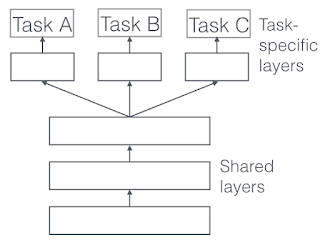
In transfer learning, you learn from a sequential process, i.e. learn from task A and transfer it to task B. However, in multi-task learning, you learn from multiple tasks simultaneously. In transfer learning, learn the NN for a big task. Then, for a smaller task just retrain the weights of the last layer only (or last 1-2 layers). You could also retrain all the parameters of the NN and in that case, it is called as pre-training because you are initializing the weights of the NN from a pre-trained model. When you are updating the weights of the model, it is also called as fine-tuning. A couple of ways in which fine tuning works is: Truncate the last layer of the NN and replace it with the new layer to learn the new output. Use a smaller learning rate to train the network. Freeze the weights of the first few layers of the NN. When does transfer learning make sense ? You have a lot of data from the task that you are originally learning from and small amount of data for the

Lets discuss this widely cited Google paper on Wide and Deep learning . The paper mentions that an important challenge in recommender systems is to achieve both memorization and generalization . Memorization is learning the frequent co-occurrence of items and features whereas generalization explores new feature combinations that have rarely occurred in the past. LR models have been widely used in Google settings and generally have sparse features with one hot encoding. Memorization and generalization can be added in such models by cross-product transformations in the feature space but require a lot of manual feature engineering. On the other hand are embedding based models that learn a low dimensional embedding for each of the categorical features. One of the problems with embedding based model is that it will lead to non-zero predictions even when the user-item matrix is high rank and consists of niche users. To solve this problem the authors present a very neat idea - use both wide

Lets first talk about the problem of one shot learning . One shot learning is learning from a single training example. This problem occurs for example in an organization where you want to recognize faces and you might have only one face of the employee. Using a convnet to output a multi-class label is not a great idea as a small training set is not enough to train a classifier and it doesn't scale to new employee joining. Instead, one way to handle this problem is to learn a similarity function between two images. One way to train the neural network to learn the similarity function is via a siamese network. The Siamese network consists of two identical neural network with same parameters so that it computes a distance function between the encodings of the two input images [Ref: DeepFace]. To define an objective function, one way is to use a triplet loss. In a triplet loss, there is an anchor image along with a positive example and a negative example (A, P, N). So what is requir

Lets next discuss a very famous NN architecture called the ResNet. One of the key questions asked in deep learning is " Would deeper networks result in higher accuracy ? " Intuitively, this may make sense but practically it is observed that the training accuracy starts to degrade with deeper networks. This is surprising as it is not caused by overfitting because we see the degradation in training error and not test error. Infact, constructing deeper networks from their shallower counterparts by just adding identity mappings also shows a similar degradation in test error. The degradation problem suggests that solvers might have difficulty in approximating identity mappings from multiple nonlinear layers. One possible causes is the problem of vanishing/exploding gradients. Resnet addresses the problem by adding residual connections or shortcut connections. Adding these connections makes it easier to learn identity mapping as: a[l+2] = g(z[l+2] + a[l]), where a[l] is the ski

Gradient descent is a way of minimizing an objective function J(θ) by updating the model's parameters in the opposite direction of the gradient of the objective function. Batch Gradient Descent : Batch gradient descent computes the gradient of the cost function for the entire training set in just one update which makes it very slow and intractable for very large datasts. The parameters are updated as follows: θ = θ - η ∇ J(θ) Batch gradient descent is guaranteed to converge to the global minimum for convex problems. Stochastic Gradient Descent : SGD performs parameter update for each training example. It is much faster and can be used to learn online but due to single point updates it can be very noisy and cause the objective function to oscillate. It can continuously keep oscillating and is not guaranteed to converge. However, upon using a decreasing learning rate it is known to converge almost certainly. Mini-batch gradient descent : This is in between the above two algori

Lets look at various different strategies for normalizing neural networks: Batch Normalization : Batch normalization is a type of layer that can adaptively normalize the data. Before we go deep in that lets first examine the phenomenon of Internal covariate shift . The change in the distribution of the internal nodes of a deep network in the course of training is called as Internal Covariate Shift. This is disadvantageous because the layers need to continuously adapt to the change in the distribution. Batch Normalization transform takes care of the problem as follows: For a layer, normalize each feature dimension as: x'(k) = x(k) - E[x(k)]/√ Var[x(k)] Simply normalizing the input can change what the layer can represent. For example, normalizing the inputs of sigmoid would constrain them to linear regime. To understand why, note that 95% of the values of a Gaussian distribution lie within the range μ ± 2σ. Hence we need to make sure that the transformation inserted in the net

Alright, next blog post lets jump quickly into some of the widely used DL models. RNNs : RNNs are a class of ANNs that process sequences. RNNs iterate through the input sequence and maintain a state of the sequence so far. Every input sequence given to the RNNs is considered independent and the state of the RNN is reset between the different inputs. From the DL book, this can be explained using the following code: W = np.random.random((output_features, input_features)) U = np.random.random((output_features, output_features)) b = np.random.random((output_features,)) output_t = np.tanh(np.dot(W, input_t) + np.dot(U, state_t) + b) state_t+1 = output_t The tanh ensures the values are between -1 and 1 and kind of acts as a regularization. LSTMs : Long Short Term Memory networks as the name suggests capture long term dependencies that the RNNs are incapable of capturing. RNNs as we saw above have a simple structure of repeating modules where each module is a single tanh layer. One of

Ok, first blog post after a loooooooong time and the first one after baby #2. Have been wanting to catch up on readings for so long and what a better way than to write it and explain it myself. Lets begin with the model which has perhaps been beaten to death in the past few years. Word2Vec is a popular algorithm to generate word embeddings. The original algorithm by Mikolov, et al. has been proposed in the following references ( 1 and 2 ). There are two key pieces of the model: The Skip-gram model: In this model, we are given a corpus of word and its context (context for example is nearby word within a window size). The goal is to train a NN to predict the probability of every word in the vocabulary given the input word (hopefully the probability of context words would be much higher). We thus need to find the parameters that maximize the probability: argmax Π p(c|w;θ) where c is the set of contexts for the word w in the corpus The conditional probability is usually paramete