Kernel SVMs
Lets now apply the idea of a dual form representation to the SVM problem to have a kernel SVM. The dual representation helps us code the problem in the form of kernels and thus is very useful to solve for non-linear problem settings. Recall that in the original formulation of the SVM, the optimization problem is as follows:
In this example, we used an RBF kernel which is infinite dimensional. Other popularly used kernels is the polynomial K(x,y) = (x.y +1)^p. The next question arises is what are the possible valid kernels ? A necessary and sufficient condition for a valid kernel is that the Gram matrix K should be positive semidefinite.
minimize 1/2|w|^2
subject to y_t(w'x + b) - 1 >= 0
This can be written in a dual form using Laggrangian and KKT conditions as follows:
J(w, b; α) minimize 1/2|w|^2 - ∑(t=1:n) αt * (y_t(w'x + b) - 1)
dJ/db = 0 =>  ∑(t=1:n) αt * y_t = 0
dJ/dw = 0 => w = ∑(t=1:n) αt * y_t * x_t = 0
Substituting it back, we get,
min ∑(i=1:n) αi - 1/2 ∑(i=1:n)∑(j=1:n)αi αj*y_i*y_j* xi'*xj
subject to ∑(i=1:n)αi = 0
This optimization is still a quadratically constrained optimization and the matlab code for classification using the RBF kernel is shown as follows:
%Generate Data
n = 50;
r1 = sqrt(rand(n,1)); % radius
t1 = 2*pi*rand(n,1);  % angle
d1 = [r1.*cos(t1) r1.*sin(t1)]; % points

r2 = sqrt(3*rand(n,1)+1); % radius
t2 = 2*pi*rand(n,1); % angle
d2 = [r2.*cos(t2), r2.*sin(t2)]; % points

x = [d1; d2];
y = [ones(n,1); -ones(n,1)];
n = 2*n;

%Construct RBF Kernel
K = zeros(n);
sig2 = 1;
for i = 1:n
    for j = i:n
        xi = x(i,:) - x(j,:);
        K(i,j) = exp( (-1/(2*sig2)) * (xi*xi') );
        K(j,i) = K(i,j);
    end
end

H = (y*y').*K;
f = -ones(n,1);
Aeq = y';
beq = 0;

%Run quadprog
qp_opts = optimset('LargeScale','Off','display','off');
[alpha, fval, exitflag, output, lambda] = ...
    quadprog(H,f,[],[],Aeq,beq, zeros(n,1), ...
    Inf*ones(n,1), ones(n,1), ...
    qp_opts);

% Find the support vectors
% calculate the parameters of the separating line from the support
% vectors.
svIndex = find(alpha > sqrt(eps));
sv = x(svIndex,:);
alphaHat = y(svIndex).*alpha(svIndex);

% Calculate the bias by applying the indicator function to the support
% vector with largest alpha.
[maxAlpha,maxPos] = max(alpha);
bias = y(maxPos) - sum(alphaHat.*K(svIndex,maxPos));

figure;
hold on;
plot(d1(:,1),d1(:,2),'r+')
plot(d2(:,1),d2(:,2),'b*')
plot(sv(:,1),sv(:,2),'ko');
axis equal

% plot decision boundary
[d1,d2] = meshgrid(-2:.1:2, -2:.1:2);
Xp = [reshape(d1,numel(d1),1) reshape(d2,numel(d2),1)];
m = length(Xp);
Z = zeros(m,1);

for i = 1:m
    xi = repmat(Xp(i,:),n,1) - x;
    xd = diag(xi * xi')';
    Kx = exp( (-1/(2*sig2)) * xd );
    Z(i) = Kx(svIndex) * alphaHat +bias;
end
contour(d1,d2,reshape(Z,size(d1,1),size(d1,2)), [0 0] ,'k');
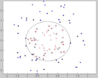
Finally, the figure showing the separation between the classes is as follows: The points that are circled are the support vectors. Note that a linear SVM would fail in such a case and using the kernel functions, we are able to get a beautiful separation in the data. 
In this example, we used an RBF kernel which is infinite dimensional. Other popularly used kernels is the polynomial K(x,y) = (x.y +1)^p. The next question arises is what are the possible valid kernels ? A necessary and sufficient condition for a valid kernel is that the Gram matrix K should be positive semidefinite.

Comments
Post a Comment