My Learnings in ML

The logistic regression method even though called regression has a unique ability to give posterior probability values for a data point to belong to a particular class and hence serve as a discriminative function useful for classification. The idea is simple, to use the logistic sigmoid function on the linear function of feature vector. p(y = 1| x) = σ(w'x +b) The likelihood function can be written as p(t|w) = Π y_i^t_i*(1 - y_i)^(1 - t_i) ln p(t|w) = Σ t_i*ln(y_i) + (1 - t_i)*ln(1 - y_i) The error function is computed by taking the negative of the log likelihood function and is computed as follows: E(w) = -ln p(t|w) Now, ∇E(w) is computed as follows: y = 1 / (1 + exp(-w'x) Taking derivative of both sides, ∇y/∇w = exp(-w'x)(x)/(1 + exp(-w'x))^2 ∇y/∇w = xy(1-y) Substituting the value in ∇E(w), we get ∇ E(w) = Σ (y_i - t_i)*x_i The derivative of the error function is similar to the least squares problem, although w...

Lets now start with another widely used tool - regression. The main goal of regression analysis is to find a function f(x) that fits the data well and predicts y from x. Also, we want to minimize the risk associated with choosing the hypothesis function. As it is difficult to measure the actual risk and minimize it, we use the empirical measure of risk and try to minimize it. Remp = 1/N ∑ Loss(y_i, f(x_i)) Least squares regression has a loss function which is basically the squared error of the target variable y_i from the predicted value f(x_i) and is defined as follows. Loss(y_i, f(x_i)) = 1/2 (y_i - f(x_i))^2 Using the above two equations and a vector representation for the input and target variable, we want to minimize the following Remp and we solve it as follows. Remp = 1/2 |y - w'X|^2 = 1/2 (y - w'X)'(y - w'X) Taking the first derivative w.r.t. w, dR/dw = d/dw 1/2 (y'y - X'wy -y'w'X +X'ww'X) = 1/2(-2X'y + 2X'Xw...

The perceptron algorithm is a linear classifier using a linear function (w'x + b) to classify the points into two classes. The loss function for the perceptron algorithm just counts the points misclassified and then incrementally adjusts the weight vector and thus the decision boundary to appropriately classify the two classes. Perhaps this is the simplest algorithm one can think of to update the weight vector and is shown as follows: w(k+1) = w(k) + yt*xt if yt ≠ f(xt; w) i.e. we cycle through the training points and adjust the weight vector only if the points are misclassified. Note that our class labels are -1 and 1 and hence if the points are misclassified then y_t* f(xt; w) will be negative. In order to understand why the seemingly simple update rule works and leads to a convergence, lets closely examine it. One of the underlying assumption in the perceptron model is that the points are linearly separated hence there exists an w* such that y_t * f(xt; w*) ≥ γ for all...

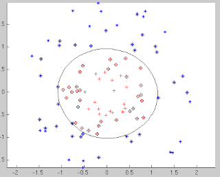
Lets now apply the idea of a dual form representation to the SVM problem to have a kernel SVM. The dual representation helps us code the problem in the form of kernels and thus is very useful to solve for non-linear problem settings. Recall that in the original formulation of the SVM, the optimization problem is as follows: minimize 1/2|w|^2 subject to y_t(w'x + b) - 1 >= 0 This can be written in a dual form using Laggrangian and KKT conditions as follows: J(w, b; α) minimize 1/2|w|^2 - ∑(t=1:n) αt * (y_t(w'x + b) - 1) dJ/db = 0 => ∑(t=1:n) αt * y_t = 0 dJ/dw = 0 => w = ∑(t=1:n) αt * y_t * x_t = 0 Substituting it back, we get, min ∑(i=1:n) αi - 1/2 ∑(i=1:n)∑(j=1:n)αi αj*y_i*y_j* xi'*xj subject to ∑(i=1:n)αi = 0 This optimization is still a quadratically constrained optimization and the matlab code for classification using the RBF kernel is shown as follows: %Generate Data n = 50; r1 = sqrt(rand(n,1)); ...

One of the popular methods for handling non-linear data using linear models is kernel methods. A kernel function essentially maps the input data into a higher dimensional space. Note that the models are still linear in the parameter space and its only the data which is mapped to a higher dimensional space. Lets consider the example of linear regression. The least squares method fits a linear function to given data by minimizing the sum of the squares of the errors made at every point. It has a closed form solution given by: w = inv(X'*X)*X'*y This solution works perfectly fine, in case the relationships in the data are linear as shown by the following example. However, consider the following example in which the relationship in the data is non-linear. The linear model fits a straight line to the data which does not capture the real relationship in the data. The least squares model can be reformulated in a dual representation leading to a kernel representation of th...

Lets begin with SVMs. SVMs are perhaps one of the most widely used classifiers. They are based upon the concept of maximizing the linear decision boundary between two classes. Let us consider a hyperplane that separates the positive and the negative classes. The points on the hyperplane H satisfy the equation w'x +b = 0. We need to maximize the separation between the two classes. Let us consider H+ and H- be the two hyperplanes that have maximum separation between them and no points from either class in between them. However, points from either of the classes do lie on the hyperplanes H+ and H-. H+ ≡ w'x +b ≥ 1 H- ≡ w'x +b ≤ -1 The distance of H+ from H = 1 -b /w and the distance of H- from H is -1 -b/w. Hence the distance between the two hyperplanes is 2/w. We want to maximize the distance or minimize w/2. More formally, we can set the optimization problem to directly maximize the decision boundary in a beautiful manner. minimize 1/2* |W|^2 subject to y_t * (w'x...